
Introduction
IceRadarAnalyzer is included with all IceRadar systems, and is a tool to review acquired radar data. Dewow/Detrend, filters, gain contol ..., and picking can be performed with the application. Data can be exported to ascii and the original hdf5 data files can also be open from Matlab, Python, or any other software environment with a HDF5 library.
System requirements
- OS: Windowns XP, 7, 10
- Monitor resolution: 1200x800 or better
- RAM: 8GB, more is better, as radardata can be quite large.
Installation
- Navigate to http://www.bluesystem.ca/downloads.html
- Once in the download page, two steps are required:
- first, and only done once, install the LabVIEW-runtime engine required for a given version of IceRadarAnalyzer, typically 2011.
- Second, download the latest IceRadarAnalyzer version zip file, extract it, and run the setup.exe
Warning
IceRadarAnalyzer is a data viewing and analysis application, and as such must not be installed on the field computer hosting the acquisition software. The radar system has a small screen to minimize the system overall size and weight, and it is too small to be used with the IceRadarAnalyzer.
Software overview
When IceRadarAnalyzer is launched, the wave parameter box pops up. These settings are required for an accurate calculation of the ice depth. Once entered, these settings can be modified at any time. These are particularly important for picking, as the depth calculation depends on it.
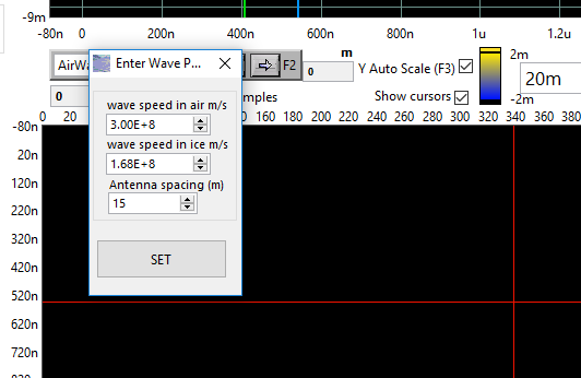
Tip
It is assumed that the medium of interst is Ice, hence, the second box heading "Wave speed in ice m/s)". If however, the radar was taken on an other medium, the radar wave velocity for this medium should be entered (ie: if a survey is conducted over a frozen lake, the media of interest is fresh water, and the wave velocity for water would be entered instead).
Viewing Data
This View Radargrams tab is the main working tab for IceRadarAnalyzer. It groups controls and indicators to view, filter and pick radar data. These specific steps will be detailed in their related sections.
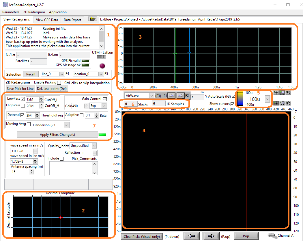
- specific line selection and locations, as well as GPS data and status bar are shown in group 1
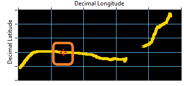
- group 2 shows GPS positions for a given line, that is the path taken on the glacier for this line. Note that the display is cartesian and some distorsion occurs with the trajectory visual rendering.
- group 3 is the plot of the one-shot radargram (stacked) for a given location as selected by the location dropdown,or the 2D plot cursors, or the red arrow from the GPS plot. On the vertical axis is a voltage as captured as the mid-point of the Rx antenna, and two-way-travel time (TWTT) on the x-axis.
- group 4, is the 2D radargram. On the left vertical axis is the TWTT, while on the right vertical axis is the corresonding depth. On the horizontal axis is the location number. Finally, on the z-axis (color scale) is the voltage as captured as the mid-point of the Rx antenna. This plot represents a 3D view of subsequent 1D plot from the 1D representation.
- the dropdown in group 5 is the z-axis scale (color scale) of the 2D radargram.
- In group 6 the number of stacks used to acquire each 1D shot is indicated, together with the number of 1D samples present in a single shot. It correspond to the vertical extent in the 2D representation plot, and horizontal extent on the 1D representation.
- this group deals with the tools used to turn a raw radargram, where details are often difficult to see, into an enhanced rendering of the original data through a set of filters and gain corrections.
Once a hdf5 file is chosen, the available lines and locations (within a line) are retrieved from the file. They are presented to the user via 2 drop downs. Selecting a Line is the next thing to do once a file is selected. The Recall button, reload the line_i indicated by the dropdown setting.
Caution
When selecting a new line, be aware that it may take 10 to 20 secs to load the data. A line can contain several 100s of MB of data.
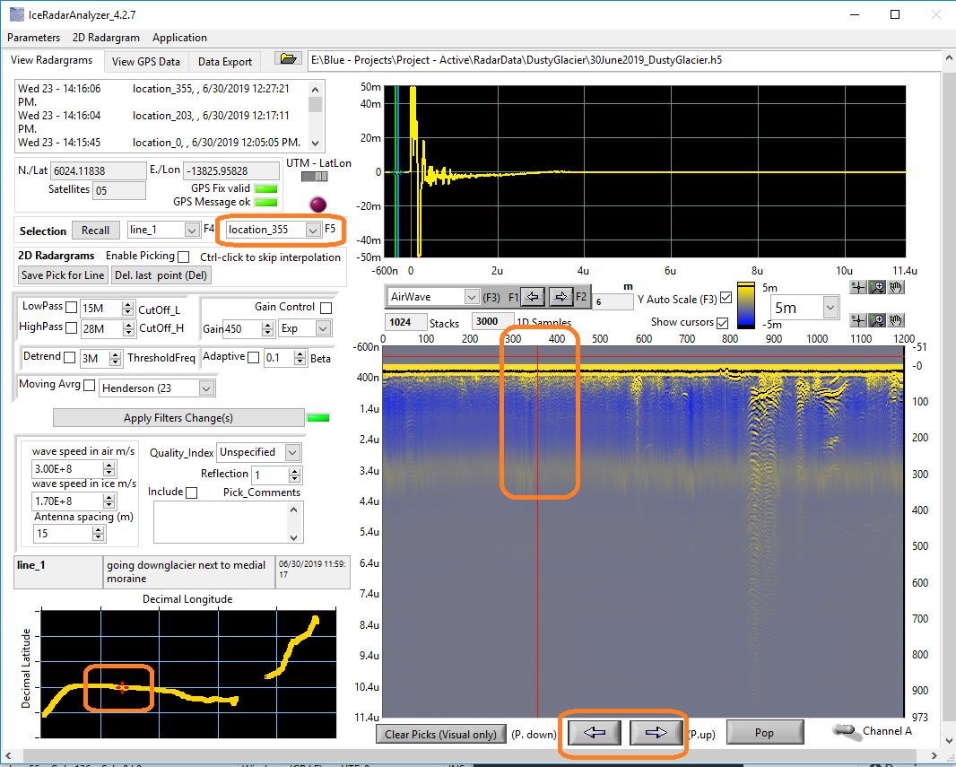
Locations can be selected from the location dropdown but it is usually more convenient to access them in the following manners:
• Selecting the Left Arrow or Right Arrow button to respectively decrement or increment the location number.
• Direcly grabing with the mouse the red crosshair on the GPS trajectory and moving it to the desired location on any other point.
• Sliding the vertical cursor on the 2D radargram view along the horizontal axis, travelling through locations.

Note
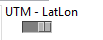
LatLon GPS data found in the raw data files are produced by the GPS unit during acquisition. UTM GPS data, if present, were added during a post processing operation on certain files. The selection switch directs the software to use one of these two sets of GPS data. If UTM data were never added, use the LatLon setting, this is the case in the vast majority of the data files, and certainly in raw datafile.
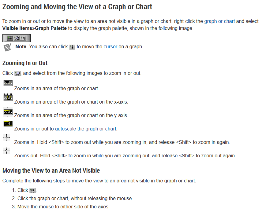
Zooming and panning
Filtering
This section describes the tools necessary to enhance the raw data rendering. Internal reflections often obscur the interesting parts of a radargram, especially when looking at raw data. This set of filters and corrections are quite helpful to address this.
-
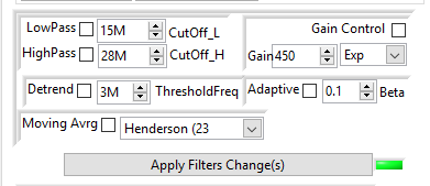
Low Pass Filter with cutoff frequency, in the example above set at 15MHz. Used very often to remove noise above the working frequency. i.e 10 MHz center frequency, LP can be set at 30 MHz. Too high and not much noise is removed, too low, and too much real signal is filtered out. Keep in mind that filters have a cut-off slope.
-
High Pass Filter Not used as often as Low Pass, as they tend to distord the signal.
-
Detrend (or Dewow) Extremelly useful to remove the low drift a radar signal often exhibits. In the above screen shots one can see the 2D radargrams show a blue hue, followed by a yellow hue. These correspond to , respectively, a slight negative offset, followed by a slight positive offset on the data (also visible on the 1D plot). The detrent threshold should be chosen well below the working frequency of the raw data to minimize distorsions.
-
Moving Average is a good filter to remove some of the noise often visible, the dropdown allows to chose a method, and more so, how many points are used to compute the average. The larger the number of points, the more averaging is taking place, at the expense of "sharpness".
All the above filters act on the TWWT time scale, so on the vertical scale of the 2D radargram. On the other hand:
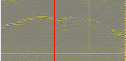
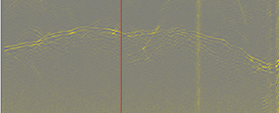
- Adaptive or memory filter, acts across radargrams on the horizontal axis from one location to the other. This filter removes or reduce the influence of invariants from one location to the other. The greater the amplitude (between 0 and 1), the greater the change between the amplitude at t-1 and t has to be so the data point at t is maintained. An example is given below where the adaptive filter is off in the upper plot, and engaged in the lower plot. Once can see that the system-related horizontal line is removed after using the adaptive filter.
Finally, the Gain Control setting applies a gain on the raw data with 2 methods:
- Exp: in this case, the gain value selected in the amplitude box is set to reach this amplitude at the end of an exponental rise starting at depth 0. So deeper amplitudes are increased more than shallower ones.
- Linear: here the gain value are increasing linearly from depth 0 to the end of the data set.
In all the above if the checkbox is selected, the correponding function is active, and to be take effect, the Apply Filter Change(s) has to be clicked.
Tip
Adjusting the vertical scale is another way to apply an equidistributed gain across data set, unlike a linear or exponental gain.
Filtering example
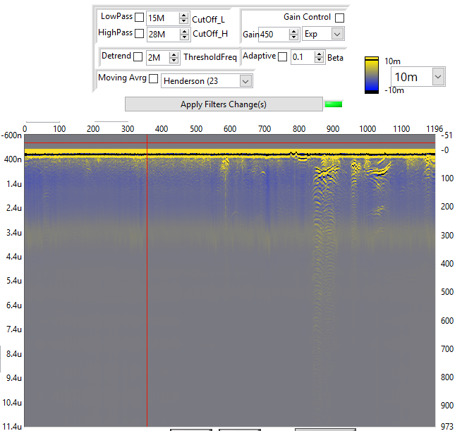
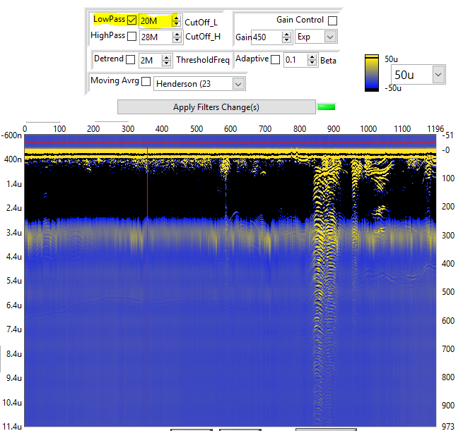
The above screenshot shows a raw dataset with neither filtering nor gain applied, and a +/- 10mV Z-axis color scale. Below, a 20 MHz low pass filter is applied (the radar working frequency was 5 MHz), and the vertical scale is set to 50 microV. A few hyperbolies are visible around 3.5 micro seconds as well as some features at around 5 microseconds towards locations [1000-1200], but the data set needs to be detrended as indicated by the string blue, black, and yellow hues.
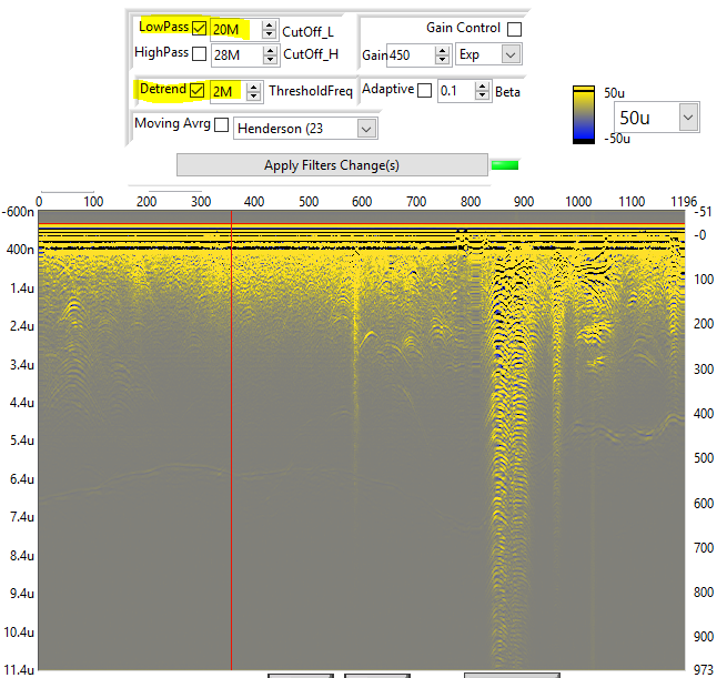
Detrending is now added below. A first hint of a reflector that could be the bed interface is now visible around 7 microseconds between locations [0-600].
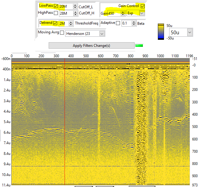
We can add an exponential gain to enhance the deeper layer preferentially. This leads to now a clear rendering of the glacier bed. The horizontal line at 9.4 micro seconds is the end of the transmitter pulse and is instrumental.
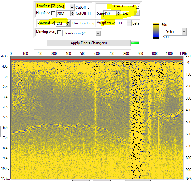
A few more steps in the filtering can help solve this and keep improving the result. First the Adaptive filter will be added with the effect of removing the invariants (horizontal line)...
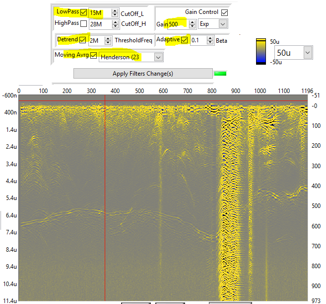
... Finally, the Moving Average is added, as well as decreasing the LP cut off to 15 MHz (hence removing more noise above the cutoff than previously), and the gain is slightly increased to 500. Once can now see the clear effects of all the filters and gain on the raw data.
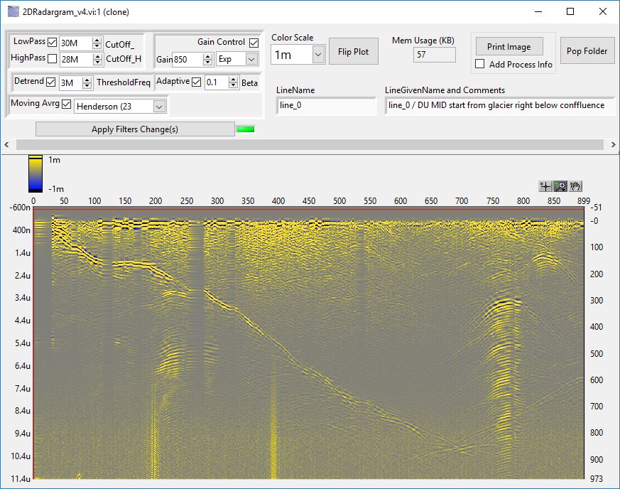
Analyzer's pop-up windows
To go further on the analysis, and to keep a processed radargram available in view on the desktop, the pop function is used.

This will pop a new analysis window with a simplified controls set mirroring the last filter settings for consistency.
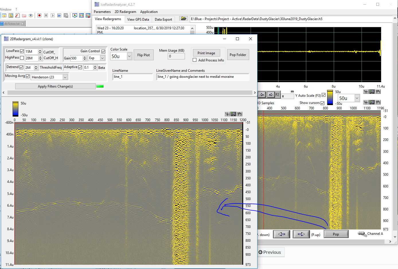
The Analyzer pop-up windows have the following features:
- Several pop-ups can be created, each with a different 2D radargram plot
- pop-ups are scalable
- filters settings are identical to the original main windows' settings and can be changed from this point on.
- the line comments are passed to the pop-up windows
- A Print Image button with an option to ** add the processing info** to the print out image (jpeg, or bmp) allows to save a the results of a specific filtering set with these settings printed over the image so they are not lost.

Picking
Note
Doc on picking is under construction...